
By: Josh Carmichael, Chris Langfield, Abhishek Biswas, and Troy Comi https://github.com/ComputationalCryoEM/ASPIRE-GPU-Hackathon
ASPIRE is an open-source Python package for 3D molecular structure determination using cryo-EM with many submodules solving complex equations that could be accelerated on GPUs. ASPIRE developers have participated in GPU hackathons for the last 4 years, but new group members Josh and Chris attended for the first time this year. The problem selected by Josh and Chris was spectral decomposition using the power method for determining leading eigenvalue/eigenvector – a limiting step in ASPIRE’s computation pipeline. The problem was ideal in scope, tested and provided a range of problem sizes for scaling experiments onto a GPU. The team primarily worked by pair programming, frequently meeting together to share paired results and determine next steps.
Resolving Python Anti-Patterns
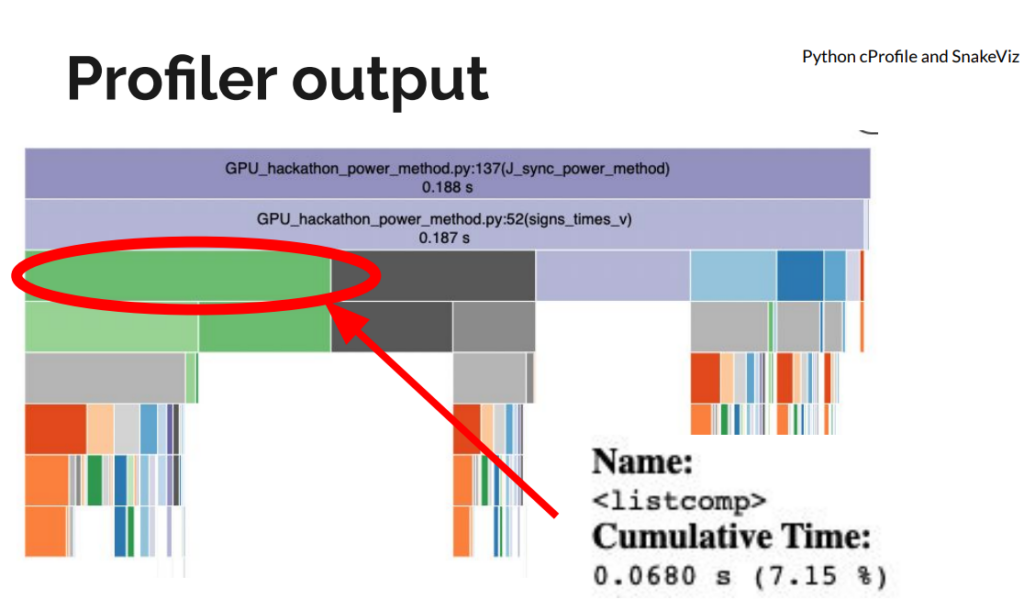
The initial implementation had a few “fast python anti-patterns”. On the first day, we replaced for-loops and Python list comprehensions with NumPy operations for large speedups, even before moving to a GPU. We used Python’s standard library profiler, cProfile to get an idea of the functions slowing down the code. We visualized the profiler output using SnakeViz.
Moving to CuPy
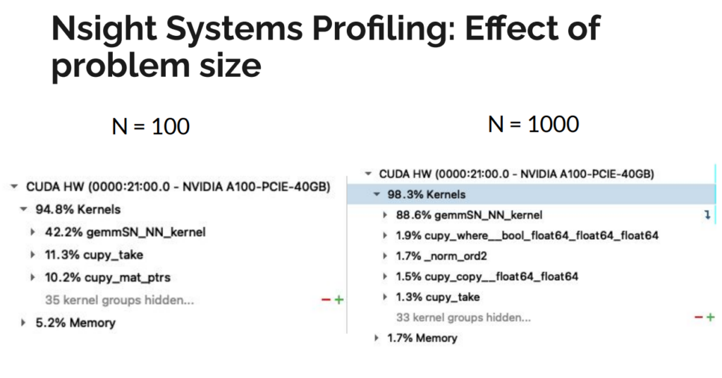
We initially used drop-in replacements of NumPy calls with CuPy. This actually worsened performance compared to a single CPU core, likely because optimizations for CPU do not necessarily translate to GPU speedups. We used NVIDIA’s Nsight Systems to generate a profile of the kernel launches being generated by CuPy and understand the memory transfers from host to device. We noticed that CuPy was generating hundreds of launches of a kernel called “gemmSN_NN_kernel”. Although each call performed a small operation, the launch time overhead was as costly as the operation itself. In aggregate, these launches added up significantly, and–worse–this issue would scale with problem size. Further analysis showed that the large number of kernel launches generated by CuPy was due primarily to two operations. First, a 4D matrix multiply was decomposed into a series of 3D multiplications, where the last dimensions were small. Flattening the matrix into 3D greatly reduced the number of kernel launches and increased the size of each operation. Second, a matrix conjugation was expressed as a direct translation of the underlying mathematical theory as two matrix multiply operations. Careful inspection of the final result revealed the costly multiplications could be replaced with a single, element-wise multiplication, further reducing the number of kernel launches performed by CuPy.
Randomizing Batch Operation
As part of refactoring, we had modified the index generator to produce subproblems in batches, instead of individually. The batch size is derived from the problem size and the indices were generated in sorted order. This caused a memory bottleneck during a final sum-reduce operation that was expressed as a weighted histogram function. The sorted indices were causing collisions into bins, leading to inefficient memory access due to the required atomicAdd when accumulating into one bin. We addressed this slowdown by randomizing the indices that are batched together to decrease the frequency of stalls during the reduce operation. We also identified that we could cache the indices for each iteration, further accelerating the code.


Figure 3: Histogram of hit counts for each iteration in the loop (a) indices generated in sorted order shows each loop updating a small number of positions causing collisions (b) randomizing the indices that are batched together decreases the frequency of stalls during the reduce operation.
Host Memory Bug
As we ramped up the problem size, we noticed that we were running out of memory on the host machine after a few iterations. Since the code was performing all operations in-place, the accumulating host memory was initially mysterious.
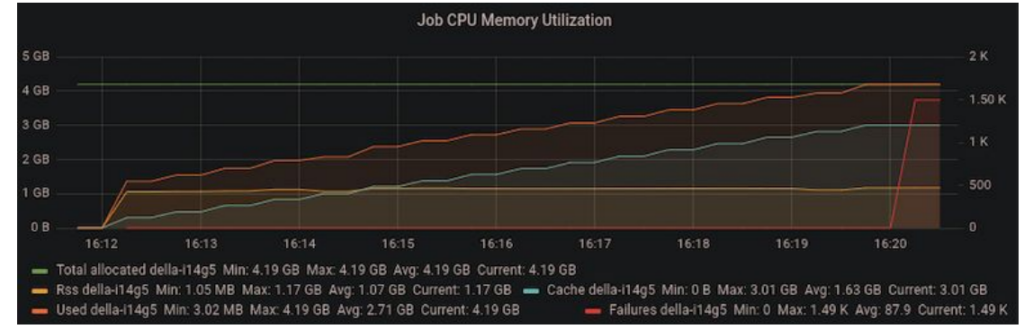
We tracked down the issue to a temporary variable overriding a variable that was used outside the loop scope in the outer iteration of the power method. In the code below, “vec” is initialized before the loop. On each iteration, “vec” is replaced with “vec_new” and the old value of “vec” can be safely discarded. However, since “vec” is used after the loop, CuPy retained a copy of “vec” on the host memory, causing copies of “vec” to accumulate.
    # Power method iterations
    for itr in range(max_iters):
        vec_new = signs_times_v(vijs, vec, conjugate, edge_signs)
        vec_new /= norm(vec_new)
        residual = norm(vec_new - vec)
        vec = vec_new
        if residual < epsilon:
            print(f'Converged after {itr} iterations of the power method.')
            break
    else:
        print('max iterations')

    # We need only the signs of the eigenvector
    J_sync = np.sign(vec)
The simple solution was to initialize vec_new before the loop and use its value after the loop exits so that CuPy knows “vec” can be safely garbage collected in each iteration.
    # initialize vec_new to prevent blocking garbage collection of vec
    vec_new = vec
    # Power method iterations
    for itr in range(max_iters):
        triplets_iter = all_triplets_batch(triplets, batch_size)
        vec_new = signs_times_v(vijs, vec, conjugate, edge_signs, triplets_iter)
        vec_new /= norm(vec_new)
        residual = norm(vec_new - vec)
        vec = vec_new
        if residual < epsilon:
            print(f'Converged after {itr} iterations of the power method.')
            break
    else:
        print('max iterations')

    # We need only the signs of the eigenvector
    J_sync = np.sign(vec_new)
Final Speedup
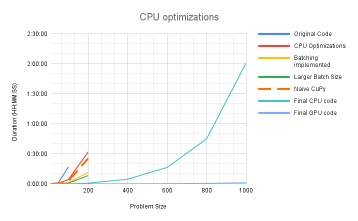
We achieved significant speedup on both CPU and the GPU. In our initial implementation the code would timeout after 4 hours, processing a problem size of N=400. After all optimizations, we are processing a realistic problem size of N=1000 in 2 hours on CPU and just over 1 minute on the GPU. The problem sizes that needed to be partitioned before can now be executed directly and the implementation is expected to scale to larger problem sizes as well.
Takeaways
There were some key points that we feel were essential to achieving these improvements within the constraints of a 4-day hackathon.
Preparation
It was crucial that the target algorithm could be run and tested in isolation, away from the rest of the codebase. Our algorithm is an intermediate step within a large computational pipeline. It would be difficult to quickly test modifications and pinpoint optimizations in the full problem context, so the algorithm was broken out of the main code and put into a standalone script. We also wrote a script to generate sample inputs of any problem size, which could be created and saved to disk outside of the code to be optimized. The key here is to identify what external information your code needs to run in a realistic setting, and try to eliminate everything else. In addition, as a sanity check, we saved *outputs* of the original code for comparison, in case our modifications unintentionally broke the code.
Don’t prematurely optimize
A lot of code is not initially written to be maximally efficient; there is often a trade-off between readability and efficiency. Correctness and communicating an algorithm are vital for code when it is first written. Look for common improvements to be made before attempting to profile the code on the GPU. For example, using cProfile we found bloated Python code that was easy to streamline without resorting to fancy solutions. Removing unnecessary list comprehensions and directly calculating indices instead of searching for them led to large speedups without sacrificing readability. Next, we optimized the code to run just on the CPU by translating verbose, multi-step calculations with more terse, single calls to NumPy routines. As a bonus, code that primarily uses NumPy is easy to translate into CuPy. Finally, we moved on to the GPU, confident that we were entering this stage of the hackathon with robust, vetted code. There are options for when code starts to become cryptic. Commenting code that has become too obtuse with the original, verbose version is an easy way to retain documentation. Moving the old version into a unit test is a more active way to ensure new versions continue to match legacy code while providing some documentation.
Working as a Group
Having two pair programming teams tackling a complicated piece of numerical code requires coordination. In addition to isolating all the code and data we needed to experiment, we put all of this into a git repository. With each pair working on an individual feature branch, along with asynchronously communicating via Slack, collisions and confusion were avoided. As mentioned above, optimization can make code more difficult to read, so verbal briefings of how and why changes were made kept everyone on the same page.