By Padraig Gleeson, Sharon Crook, David Turner, Katherine Mantel, Mayank Raunak, Ted Willke, Jonathan D. Cohen
Neuroscience, cognitive science, and computer science are increasingly benefiting through their interactions. This could be accelerated by direct sharing of computational models across disparate modeling software used in each. We describe a Model Description Format designed to meet this challenge.
By Robert LeDesma, Brigitte Heller, Abhishek Biswas, Stephanie Maya, Stefania Gili, John Higgins, Alexander Ploss
Hepatitis E virus (HEV) is an RNA virus responsible for over 20 million infections annually. HEV’s open reading frame (ORF)1 polyprotein is essential for genome replication, though it is unknown how the different subdomains function within a structural context. Our data show that ORF1 operates as a multifunctional protein, which is not subject to proteolytic processing. Supporting this model, scanning mutagenesis performed on the putative papain-like cysteine protease (pPCP) domain revealed six cysteines essential for viral replication. Our data are consistent with their role in divalent metal ion coordination, which governs local and interdomain interactions that are critical for the overall structure of ORF1; furthermore, the ‘pPCP’ domain can only rescue viral genome replication in trans when expressed in the context of the full-length ORF1 protein but not as an individual subdomain. Taken together, our work provides a comprehensive model of the structure and function of HEV ORF1.
By Tamura T, Zhang J, Madan V, Biswas A, Schwoerer MP, Cafiero TR, Heller BL, Wang W, Ploss A.
Dengue is caused by four genetically distinct viral serotypes, dengue virus (DENV) 1-4. Following transmission by Aedes mosquitoes, DENV can cause a broad spectrum of clinically apparent disease ranging from febrile illness to dengue hemorrhagic fever and dengue shock syndrome. Progress in the understanding of different dengue serotypes and their impacts on specific host-virus interactions has been hampered by the scarcity of tools that adequately reflect their antigenic and genetic diversity. To bridge this gap, we created and characterized infectious clones of DENV1-4 originating from South America, Africa, and Southeast Asia. Analysis of whole viral genome sequences of five DENV isolates from each of the four serotypes confirmed their broad genetic and antigenic diversity. Using a modified circular polymerase extension reaction (CPER), we generated de novo viruses from these isolates. The resultant clones replicated robustly in human and insect cells at levels similar to those of the parental strains. To investigate in vivo properties of these genetically diverse isolates, representative viruses from each DENV serotype were administered to NOD Rag1-/-, IL2rgnull Flk2-/- (NRGF) mice, engrafted with components of a human immune system. All DENV strains tested resulted in viremia in humanized mice and induced cellular and IgM immune responses. Collectively, we describe here a workflow for rapidly generating de novo infectious clones of DENV – and conceivably other RNA viruses. The infectious clones described here are a valuable resource for reverse genetic studies and for characterizing host responses to DENV in vitro and in vivo.
ASPIRE is an open-source Python package for 3D molecular structure determination using cryo-EM with many submodules solving complex equations that could be accelerated on GPUs. ASPIRE developers have participated in GPU hackathons for the last 4 years, but new group members Josh and Chris attended for the first time this year. The problem selected by Josh and Chris was spectral decomposition using the power method for determining leading eigenvalue/eigenvector – a limiting step in ASPIRE’s computation pipeline. The problem was ideal in scope, tested and provided a range of problem sizes for scaling experiments onto a GPU. The team primarily worked by pair programming, frequently meeting together to share paired results and determine next steps.
Resolving Python Anti-Patterns
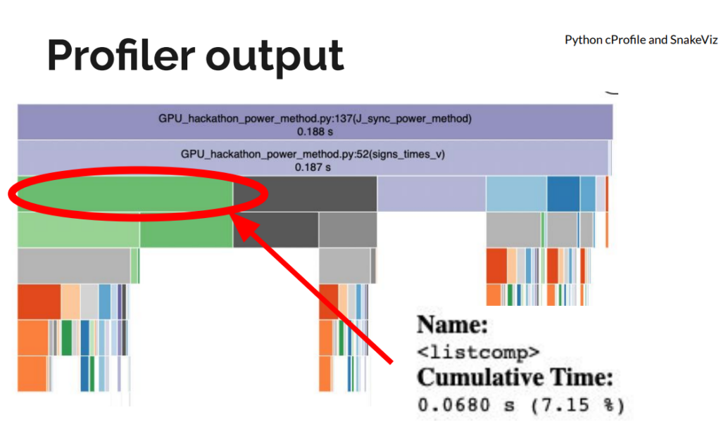
The initial implementation had a few “fast python anti-patterns”. On the first day, we replaced for-loops and Python list comprehensions with NumPy operations for large speedups, even before moving to a GPU. We used Python’s standard library profiler, cProfile to get an idea of the functions slowing down the code. We visualized the profiler output using SnakeViz.
Figure 1: Python cProfile of the original implementation visualized with SnakeViz.
Moving to CuPy
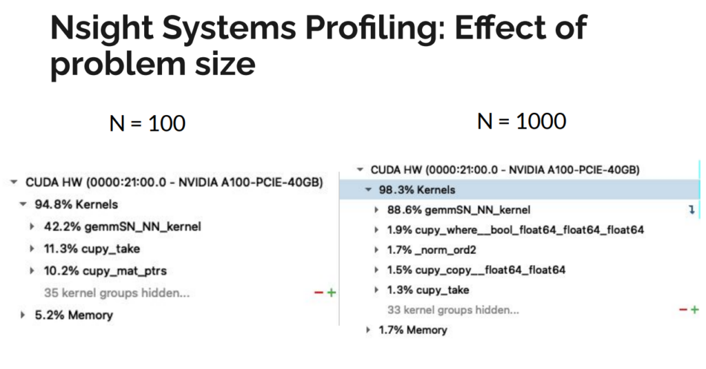
We initially used drop-in replacements of NumPy calls with CuPy. This actually worsened performance compared to a single CPU core, likely because optimizations for CPU do not necessarily translate to GPU speedups. We used NVIDIA’s Nsight Systems to generate a profile of the kernel launches being generated by CuPy and understand the memory transfers from host to device. We noticed that CuPy was generating hundreds of launches of a kernel called “gemmSN_NN_kernel”. Although each call performed a small operation, the launch time overhead was as costly as the operation itself. In aggregate, these launches added up significantly, and–worse–this issue would scale with problem size. Further analysis showed that the large number of kernel launches generated by CuPy was due primarily to two operations. First, a 4D matrix multiply was decomposed into a series of 3D multiplications, where the last dimensions were small. Flattening the matrix into 3D greatly reduced the number of kernel launches and increased the size of each operation. Second, a matrix conjugation was expressed as a direct translation of the underlying mathematical theory as two matrix multiply operations. Careful inspection of the final result revealed the costly multiplications could be replaced with a single, element-wise multiplication, further reducing the number of kernel launches performed by CuPy.
Figure 2: Nvidia Nsight Systems breakdown of naive drop-in CuPy replacement showing costly matrix multiply kernel launches.
Randomizing Batch Operation
As part of refactoring, we had modified the index generator to produce subproblems in batches, instead of individually. The batch size is derived from the problem size and the indices were generated in sorted order. This caused a memory bottleneck during a final sum-reduce operation that was expressed as a weighted histogram function. The sorted indices were causing collisions into bins, leading to inefficient memory access due to the required atomicAdd when accumulating into one bin. We addressed this slowdown by randomizing the indices that are batched together to decrease the frequency of stalls during the reduce operation. We also identified that we could cache the indices for each iteration, further accelerating the code.
Figure 3: Histogram of hit counts for each iteration in the loop (a) indices generated in sorted order shows each loop updating a small number of positions causing collisions (b) randomizing the indices that are batched together decreases the frequency of stalls during the reduce operation.
Host Memory Bug
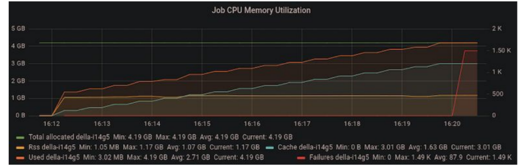
As we ramped up the problem size, we noticed that we were running out of memory on the host machine after a few iterations. Since the code was performing all operations in-place, the accumulating host memory was initially mysterious.
Figure 4: Increasing memory utilization in the host machine suggesting a memory leak.
We tracked down the issue to a temporary variable overriding a variable that was used outside the loop scope in the outer iteration of the power method. In the code below, “vec” is initialized before the loop. On each iteration, “vec” is replaced with “vec_new” and the old value of “vec” can be safely discarded. However, since “vec” is used after the loop, CuPy retained a copy of “vec” on the host memory, causing copies of “vec” to accumulate.
    # Power method iterations
    for itr in range(max_iters):
        vec_new = signs_times_v(vijs, vec, conjugate, edge_signs)
        vec_new /= norm(vec_new)
        residual = norm(vec_new - vec)
        vec = vec_new
        if residual < epsilon:
            print(f'Converged after {itr} iterations of the power method.')
            break
    else:
        print('max iterations')

    # We need only the signs of the eigenvector
    J_sync = np.sign(vec)
The simple solution was to initialize vec_new before the loop and use its value after the loop exits so that CuPy knows “vec” can be safely garbage collected in each iteration.
# initialize vec_new to prevent blocking garbage collection of vecvec_new = vec
# Power method iterations
for itr in range(max_iters):
triplets_iter = all_triplets_batch(triplets, batch_size)
vec_new = signs_times_v(vijs, vec, conjugate, edge_signs, triplets_iter)
vec_new /= norm(vec_new)
residual = norm(vec_new - vec)
vec = vec_new
if residual < epsilon:
print(f'Converged after {itr} iterations of the power method.')
break
else:
print('max iterations')
# We need only the signs of the eigenvector
J_sync = np.sign(vec_new)
Final Speedup
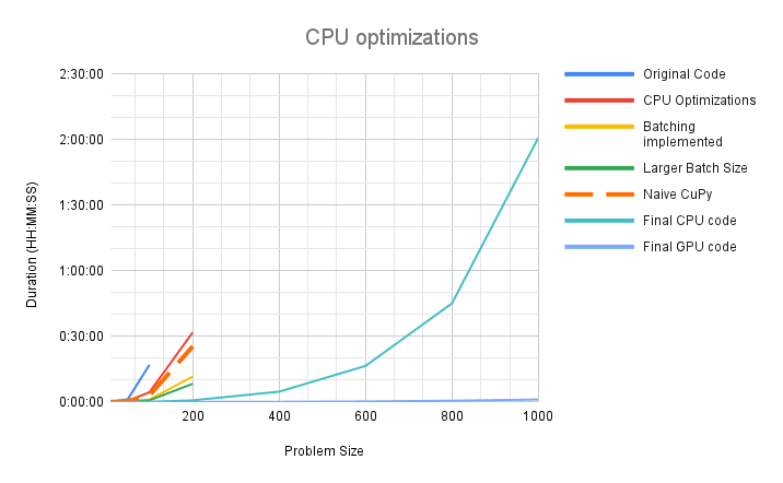
We achieved significant speedup on both CPU and the GPU. In our initial implementation the code would timeout after 4 hours, processing a problem size of N=400. After all optimizations, we are processing a realistic problem size of N=1000 in 2 hours on CPU and just over 1 minute on the GPU. The problem sizes that needed to be partitioned before can now be executed directly and the implementation is expected to scale to larger problem sizes as well.
Figure 5: Performance scaling chart showing improvement in both the serial and GPU versions. The serial version is estimated to have 30x speedup over the original version and the GPU accelerated version has a further speedup of 120x over the serial version.
Takeaways
There were some key points that we feel were essential to achieving these improvements within the constraints of a 4-day hackathon.
Preparation
It was crucial that the target algorithm could be run and tested in isolation, away from the rest of the codebase. Our algorithm is an intermediate step within a large computational pipeline. It would be difficult to quickly test modifications and pinpoint optimizations in the full problem context, so the algorithm was broken out of the main code and put into a standalone script. We also wrote a script to generate sample inputs of any problem size, which could be created and saved to disk outside of the code to be optimized. The key here is to identify what external information your code needs to run in a realistic setting, and try to eliminate everything else. In addition, as a sanity check, we saved *outputs* of the original code for comparison, in case our modifications unintentionally broke the code.
Don’t prematurely optimize
A lot of code is not initially written to be maximally efficient; there is often a trade-off between readability and efficiency. Correctness and communicating an algorithm are vital for code when it is first written. Look for common improvements to be made before attempting to profile the code on the GPU. For example, using cProfile we found bloated Python code that was easy to streamline without resorting to fancy solutions. Removing unnecessary list comprehensions and directly calculating indices instead of searching for them led to large speedups without sacrificing readability. Next, we optimized the code to run just on the CPU by translating verbose, multi-step calculations with more terse, single calls to NumPy routines. As a bonus, code that primarily uses NumPy is easy to translate into CuPy. Finally, we moved on to the GPU, confident that we were entering this stage of the hackathon with robust, vetted code. There are options for when code starts to become cryptic. Commenting code that has become too obtuse with the original, verbose version is an easy way to retain documentation. Moving the old version into a unit test is a more active way to ensure new versions continue to match legacy code while providing some documentation.
Working as a Group
Having two pair programming teams tackling a complicated piece of numerical code requires coordination. In addition to isolating all the code and data we needed to experiment, we put all of this into a git repository. With each pair working on an individual feature branch, along with asynchronously communicating via Slack, collisions and confusion were avoided. As mentioned above, optimization can make code more difficult to read, so verbal briefings of how and why changes were made kept everyone on the same page.
By Talmo D. Pereira, Nathaniel Tabris, Arie Matsliah, David M. Turner, Junyu Li, Shruthi Ravindranath, Eleni S. Papadoyannis, Edna Normand, David S. Deutsch, Z. Yan Wang, Grace C. McKenzie-Smith, Catalin C. Mitelut, Marielisa Diez Castro, John D’Uva, Mikhail Kislin, Dan H. Sanes, Sarah D. Kocher, Samuel S.-H. Wang, Annegret L. Falkner, Joshua W. Shaevitz & Mala Murthy
The desire to understand how the brain generates and patterns behavior has driven rapid methodological innovation in tools to quantify natural animal behavior. While advances in deep learning and computer vision have enabled markerless pose estimation in individual animals, extending these to multiple animals presents unique challenges for studies of social behaviors or animals in their natural environments. Here we present Social LEAP Estimates Animal Poses (SLEAP), a machine learning system for multi-animal pose tracking. This system enables versatile workflows for data labeling, model training and inference on previously unseen data. SLEAP features an accessible graphical user interface, a standardized data model, a reproducible configuration system, over 30 model architectures, two approaches to part grouping and two approaches to identity tracking. We applied SLEAP to seven datasets across flies, bees, mice and gerbils to systematically evaluate each approach and architecture, and we compare it with other existing approaches. SLEAP achieves greater accuracy and speeds of more than 800 frames per second, with latencies of less than 3.5 ms at full 1,024 × 1,024 image resolution. This makes SLEAP usable for real-time applications, which we demonstrate by controlling the behavior of one animal on the basis of the tracking and detection of social interactions with another animal.
Manoj Kumar, Michael J. Anderson, James W. Antony, Christopher Baldassano, Paula P. Brooks, Ming Bo Cai, Po-Hsuan Cameron Chen, Cameron T. Ellis, Gregory Henselman-Petrusek, David Huberdeau, J. Benjamin Hutchinson, Y. Peeta Li, Qihong Lu, Jeremy R. Manning, Anne C. Mennen, Samuel A. Nastase, Hugo Richard, Anna C. Schapiro, Nicolas W. Schuck, Michael Shvartsman, Narayanan Sundaram, Daniel Suo, Javier S. Turek, David Turner, Vy A. Vo, Grant Wallace, Yida Wang, Jamal A. Williams, Hejia Zhang, Xia Zhu, Mihai Capota˘, Jonathan D. Cohen, Uri Hasson, Kai Li, Peter J. Ramadge, Nicholas B. Turk-Browne, Theodore L. Willke, Kenneth A. Norman
Functional magnetic resonance imaging (fMRI) offers a rich source of data for studying the neural basis of cognition. Here, we describe the Brain Imaging Analysis Kit (BrainIAK), an open-source, free Python package that provides computationally optimized solutions to key problems in advanced fMRI analysis. A variety of techniques are presently included in BrainIAK: intersubject correlation (ISC) and intersubject functional connectivity (ISFC), functional alignment via the shared response model (SRM), full correlation matrix analysis (FCMA), a Bayesian version of representational similarity analysis (BRSA), event segmentation using hidden Markov models, topographic factor analysis (TFA), inverted encoding models (IEMs), an fMRI data simulator that uses noise characteristics from real data (fmrisim), and some emerging methods. These techniques have been optimized to leverage the efficiencies of high-performance compute (HPC) clusters, and the same code can be seamlessly transferred from a laptop to a cluster. For each of the aforementioned techniques, we describe the data analysis problem that the technique is meant to solve and how it solves that problem; we also include an example Jupyter notebook for each technique and an annotated bibliography of papers that have used and/or described that technique. In addition to the sections describing various analysis techniques in BrainIAK, we have included sections describing the future applications of BrainIAK to real-time fMRI, tutorials that we have developed and shared online to facilitate learning the techniques in BrainIAK, computational innovations in BrainIAK, and how to contribute to BrainIAK. We hope that this manuscript helps readers to understand how BrainIAK might be useful in their research.
By Tran, H.; Leonarduzzi, E.; De la Fuente, L.; Hull, R.B.; Bansal, V.; Chennault, C.; Gentine, P.; Melchior, P.; Condon, L.E.; Maxwell, R.M.
Integrated hydrologic models solve coupled mathematical equations that represent natural processes, including groundwater, unsaturated, and overland flow. However, these models are computationally expensive. It has been recently shown that machine leaning (ML) and deep learning (DL) in particular could be used to emulate complex physical processes in the earth system. In this study, we demonstrate how a DL model can emulate transient, three-dimensional integrated hydrologic model simulations at a fraction of the computational expense. This emulator is based on a DL model previously used for modeling video dynamics, PredRNN. The emulator is trained based on physical parameters used in the original model, inputs such as hydraulic conductivity and topography, and produces spatially distributed outputs (e.g., pressure head) from which quantities such as streamflow and water table depth can be calculated. Simulation results from the emulator and ParFlow agree well with average relative biases of 0.070, 0.092, and 0.032 for streamflow, water table depth, and total water storage, respectively. Moreover, the emulator is up to 42 times faster than ParFlow. Given this promising proof of concept, our results open the door to future applications of full hydrologic model emulation, particularly at larger scales.
By Balaich J, Estrella M, Wu G, Jeffrey PD, Biswas A, Zhao L, Korennykh A, Donia MS
The human microbiome encodes a large repertoire of biochemical enzymes and pathways, most of which remain uncharacterized. Here, using a metagenomics-based search strategy, we discovered that bacterial members of the human gut and oral microbiome encode enzymes that selectively phosphorylate a clinically used antidiabetic drug, acarbose1,2, resulting in its inactivation. Acarbose is an inhibitor of both human and bacterial α-glucosidases3, limiting the ability of the target organism to metabolize complex carbohydrates. Using biochemical assays, X-ray crystallography and metagenomic analyses, we show that microbiome-derived acarbose kinases are specific for acarbose, provide their harbouring organism with a protective advantage against the activity of acarbose, and are widespread in the microbiomes of western and non-western human populations. These results provide an example of widespread microbiome resistance to a non-antibiotic drug, and suggest that acarbose resistance has disseminated in the human microbiome as a defensive strategy against a potential endogenous producer of a closely related molecule.
By Lena P. Basta, Michael Hill-Oliva, Sarah V. Paramore, Rishabh Sharan, Audrey Goh, Abhishek Biswas, Marvin Cortez, Katherine A. Little, Eszter Posfai, Danelle Devenport
The collective polarization of cellular structures and behaviors across a tissue plane is a near universal feature of epithelia known as planar cell polarity (PCP). This property is controlled by the core PCP pathway, which consists of highly conserved membrane-associated protein complexes that localize asymmetrically at cell junctions. Here, we introduce three new mouse models for investigating the localization and dynamics of transmembrane PCP proteins: Celsr1, Fz6 and Vangl2. Using the skin epidermis as a model, we characterize and verify the expression, localization and function of endogenously tagged Celsr1-3xGFP, Fz6-3xGFP and tdTomato-Vangl2 fusion proteins. Live imaging of Fz6-3xGFP in basal epidermal progenitors reveals that the polarity of the tissue is not fixed through time. Rather, asymmetry dynamically shifts during cell rearrangements and divisions, while global, average polarity of the tissue is preserved. We show using super-resolution STED imaging that Fz6-3xGFP and tdTomato-Vangl2 can be resolved, enabling us to observe their complex localization along junctions. We further explore PCP fusion protein localization in the trachea and neural tube, and discover new patterns of PCP expression and localization throughout the mouse embryo.
By Yu-hsuan Shih, Garrett Wright, Joakim Andén, Johannes Blaschke, Alex H. Barnett
Nonuniform fast Fourier transforms dominate the computational cost in many applications including image reconstruction and signal processing. We thus present a general-purpose GPU-based CUDA library for type 1 (nonuniform to uniform) and type 2 (uniform to nonuniform) transforms in dimensions 2 and 3, in single or double precision. It achieves high performance for a given user-requested accuracy, regardless of the distribution of nonuniform points, via cache-aware point reordering, and load-balanced blocked spreading in shared memory. At low accuracies, this gives on-GPU throughputs around 10e9 nonuniform points per second, and (even including host-device transfer) is typically 4-10x faster than the latest parallel CPU code FINUFFT (at 28 threads). It is competitive with two established GPU codes, being up to 90x faster at high accuracy and/or type 1 clustered point distributions. Finally we demonstrate a 5-12x speedup versus CPU in an X-ray diffraction 3D iterative reconstruction task at 10e-12 accuracy, observing excellent multi-GPU weak scaling up to one rank per GPU.